Extracting Efficiencies and MTRs
Source:vignettes/efficiency-extraction.Rmd
efficiency-extraction.RmdOverview
Once a metafrontier model has been fitted, a range of S3
methods are available to extract and inspect results. This vignette
demonstrates all of them using a simple sfacross + LP
example.
Setup: Fit a Model
library(smfa)
#> Loading required package: sfaR
#>            ****           *******
#>           /**/           /**////**
#>   ****** ******  ******  /**   /**
#>  **//// ///**/  //////** /*******
#> //*****   /**    ******* /**///**
#>  /////**  /**   **////** /**  //**
#>  ******   /**  //********/**   //**
#> //////    //    //////// //     //    version 1.0.1
#>
#> * Please cite the 'sfaR' package as:
#>   Dakpo KH., Desjeux Y., Henningsen A., and Latruffe L. (2024). sfaR: Stochastic Frontier Analysis Using R. R package version 1.0.1.
#>
#> See also: citation("sfaR")
#>
#> * For any questions, suggestions, or comments on the 'sfaR' package, you can contact directly the authors or visit:  https://github.com/hdakpo/sfaR/issues
#>                         .d888
#>                        d88P"
#>                        888
#> .d8888b  88888b.d88b.  888888 8888b.
#> 88K      888 "888 "88b 888       "88b
#>  Y8888b. 888  888  888 888   .d888888
#>      X88 888  888  888 888   888  888
#>  88888P' 888  888  888 888   "Y888888
#>                           version 1.0.1
#>
#> * Please cite the 'smfa' package as:
#> Owili, SO. (2026). smfa: Stochastic Metafrontier Analysis. R package version 1.0.1.
#>
#> See also: citation("smfa")
#>
#> * For any questions, suggestions, or comments on the 'smfa' package, you can contact the authors directly or visit:
#>   https://github.com/SulmanOlieko/smfa/issues
data("ricephil", package = "sfaR")

ricephil$group <- cut(
  ricephil$AREA,
  breaks        = quantile(ricephil$AREA, probs = c(0, 1/3, 2/3, 1), na.rm = TRUE),
  labels        = c("small", "medium", "large"),
  include.lowest = TRUE
)

meta_lp <- smfa(
  formula    = log(PROD) ~ log(AREA) + log(LABOR) + log(NPK),
  data       = ricephil,
  group      = "group",
  S          = 1,
  udist      = "hnormal",
  groupType  = "sfacross",
  metaMethod = "lp"
)
summary() — Full Model Summary
Prints the complete model output including group-specific SFA results, metafrontier coefficients (if available), and efficiency statistics by group.
summary(meta_lp)Toggle to see the output
#> ============================================================
#> Stochastic Metafrontier Analysis
#> Metafrontier method: Linear Programming (LP) Metafrontier
#> Stochastic Production/Profit Frontier, e = v - u
#> Group approach     : Stochastic Frontier Analysis
#> Group estimator    : sfacross
#> Group optim solver : BFGS maximization
#> Groups ( 3 ): small, medium, large
#> Total observations : 344
#> Distribution       : hnormal
#> ============================================================
#>
#> ------------------------------------------------------------
#> Group: small (N = 125)  Log-likelihood: -50.98578
#> ------------------------------------------------------------
#> --------------------------------------------------------------------------------
#> Normal-Half Normal SF Model
#> Dependent Variable:                                                    log(PROD)
#> Log likelihood solver:                                         BFGS maximization
#> Log likelihood iter:                                                          42
#> Log likelihood value:                                                  -50.98578
#> Log likelihood gradient norm:                                        9.40653e-06
#> Estimation based on:                                         N =  125 and K =  6
#> Inf. Cr:                                           AIC  =  114.0 AIC/N  =  0.912
#>                                                    BIC  =  130.9 BIC/N  =  1.048
#>                                                    HQIC =  120.9 HQIC/N =  0.967
#> --------------------------------------------------------------------------------
#> Variances: Sigma-squared(v)   =                                          0.05318
#>            Sigma(v)           =                                          0.05318
#>            Sigma-squared(u)   =                                          0.23435
#>            Sigma(u)           =                                          0.23435
#> Sigma = Sqrt[(s^2(u)+s^2(v))] =                                          0.53622
#> Gamma = sigma(u)^2/sigma^2    =                                          0.81504
#> Lambda = sigma(u)/sigma(v)    =                                          2.09921
#> Var[u]/{Var[u]+Var[v]}        =                                          0.61558
#> --------------------------------------------------------------------------------
#> Average inefficiency E[ui]     =                                         0.38626
#> Average efficiency E[exp(-ui)] =                                         0.70643
#> --------------------------------------------------------------------------------
#> Stochastic Production/Profit Frontier, e = v - u
#> -----[ Tests vs. No Inefficiency ]-----
#> Likelihood Ratio Test of Inefficiency
#> Deg. freedom for inefficiency model                                            1
#> Log Likelihood for OLS Log(H0) =                                       -54.80277
#> LR statistic:
#> Chisq = 2*[LogL(H0)-LogL(H1)]  =                                         7.63398
#> Kodde-Palm C*:       95%: 2.70554                                   99%: 5.41189
#> Coelli (1995) skewness test on OLS residuals
#> M3T: z                         =                                        -3.57676
#> M3T: p.value                   =                                         0.00035
#> Final maximum likelihood estimates
#> --------------------------------------------------------------------------------
#>                          Deterministic Component of SFA
#> --------------------------------------------------------------------------------
#>                Coefficient Std. Error z value  Pr(>|z|)
#> (Intercept)       -1.58745    0.51274 -3.0960  0.001962 **
#> log(AREA)          0.24014    0.11834  2.0292  0.042440 *
#> log(LABOR)         0.43464    0.12292  3.5361  0.000406 ***
#> log(NPK)           0.30516    0.05701  5.3523 8.682e-08 ***
#> --------------------------------------------------------------------------------
#>                   Parameter in variance of u (one-sided error)
#> --------------------------------------------------------------------------------
#>                Coefficient Std. Error z value  Pr(>|z|)
#> Zu_(Intercept)    -1.45093    0.29867  -4.858 1.186e-06 ***
#> --------------------------------------------------------------------------------
#>                  Parameters in variance of v (two-sided error)
#> --------------------------------------------------------------------------------
#>                Coefficient Std. Error z value  Pr(>|z|)
#> Zv_(Intercept)    -2.93406    0.35401  -8.288 < 2.2e-16 ***
#> ---
#> Signif. codes:  0 '***' 0.001 '**' 0.01 '*' 0.05 '.' 0.1 ' ' 1
#> --------------------------------------------------------------------------------
#> Model was estimated on : Jul Tue 14, 2026 at 21:26
#> Log likelihood status: successful convergence
#> --------------------------------------------------------------------------------
#>
#> ------------------------------------------------------------
#> Group: medium (N = 104)  Log-likelihood: -15.28164
#> ------------------------------------------------------------
#> --------------------------------------------------------------------------------
#> Normal-Half Normal SF Model
#> Dependent Variable:                                                    log(PROD)
#> Log likelihood solver:                                         BFGS maximization
#> Log likelihood iter:                                                          41
#> Log likelihood value:                                                  -15.28164
#> Log likelihood gradient norm:                                        3.83566e-05
#> Estimation based on:                                         N =  104 and K =  6
#> Inf. Cr:                                            AIC  =  42.6 AIC/N  =  0.409
#>                                                     BIC  =  58.4 BIC/N  =  0.562
#>                                                     HQIC =  49.0 HQIC/N =  0.471
#> --------------------------------------------------------------------------------
#> Variances: Sigma-squared(v)   =                                          0.01058
#>            Sigma(v)           =                                          0.01058
#>            Sigma-squared(u)   =                                          0.22010
#>            Sigma(u)           =                                          0.22010
#> Sigma = Sqrt[(s^2(u)+s^2(v))] =                                          0.48030
#> Gamma = sigma(u)^2/sigma^2    =                                          0.95412
#> Lambda = sigma(u)/sigma(v)    =                                          4.56034
#> Var[u]/{Var[u]+Var[v]}        =                                          0.88314
#> --------------------------------------------------------------------------------
#> Average inefficiency E[ui]     =                                         0.37433
#> Average efficiency E[exp(-ui)] =                                         0.71330
#> --------------------------------------------------------------------------------
#> Stochastic Production/Profit Frontier, e = v - u
#> -----[ Tests vs. No Inefficiency ]-----
#> Likelihood Ratio Test of Inefficiency
#> Deg. freedom for inefficiency model                                            1
#> Log Likelihood for OLS Log(H0) =                                       -21.11323
#> LR statistic:
#> Chisq = 2*[LogL(H0)-LogL(H1)]  =                                        11.66318
#> Kodde-Palm C*:       95%: 2.70554                                   99%: 5.41189
#> Coelli (1995) skewness test on OLS residuals
#> M3T: z                         =                                        -2.91021
#> M3T: p.value                   =                                         0.00361
#> Final maximum likelihood estimates
#> --------------------------------------------------------------------------------
#>                          Deterministic Component of SFA
#> --------------------------------------------------------------------------------
#>                Coefficient Std. Error z value  Pr(>|z|)
#> (Intercept)       -0.08182    0.50668 -0.1615 0.8717190
#> log(AREA)          0.47410    0.13984  3.3903 0.0006981 ***
#> log(LABOR)         0.17935    0.10201  1.7581 0.0787310 .
#> log(NPK)           0.20255    0.08130  2.4913 0.0127289 *
#> --------------------------------------------------------------------------------
#>                   Parameter in variance of u (one-sided error)
#> --------------------------------------------------------------------------------
#>                Coefficient Std. Error z value  Pr(>|z|)
#> Zu_(Intercept)    -1.51367    0.23549 -6.4276 1.296e-10 ***
#> --------------------------------------------------------------------------------
#>                  Parameters in variance of v (two-sided error)
#> --------------------------------------------------------------------------------
#>                Coefficient Std. Error z value  Pr(>|z|)
#> Zv_(Intercept)    -4.54846    0.76429 -5.9512 2.661e-09 ***
#> ---
#> Signif. codes:  0 '***' 0.001 '**' 0.01 '*' 0.05 '.' 0.1 ' ' 1
#> --------------------------------------------------------------------------------
#> Model was estimated on : Jul Tue 14, 2026 at 21:26
#> Log likelihood status: successful convergence
#> --------------------------------------------------------------------------------
#>
#> ------------------------------------------------------------
#> Group: large (N = 115)  Log-likelihood: -8.02197
#> ------------------------------------------------------------
#> --------------------------------------------------------------------------------
#> Normal-Half Normal SF Model
#> Dependent Variable:                                                    log(PROD)
#> Log likelihood solver:                                         BFGS maximization
#> Log likelihood iter:                                                          68
#> Log likelihood value:                                                   -8.02197
#> Log likelihood gradient norm:                                        4.01301e-05
#> Estimation based on:                                         N =  115 and K =  6
#> Inf. Cr:                                            AIC  =  28.0 AIC/N  =  0.244
#>                                                     BIC  =  44.5 BIC/N  =  0.387
#>                                                     HQIC =  34.7 HQIC/N =  0.302
#> --------------------------------------------------------------------------------
#> Variances: Sigma-squared(v)   =                                          0.01399
#>            Sigma(v)           =                                          0.01399
#>            Sigma-squared(u)   =                                          0.16751
#>            Sigma(u)           =                                          0.16751
#> Sigma = Sqrt[(s^2(u)+s^2(v))] =                                          0.42602
#> Gamma = sigma(u)^2/sigma^2    =                                          0.92293
#> Lambda = sigma(u)/sigma(v)    =                                          3.46063
#> Var[u]/{Var[u]+Var[v]}        =                                          0.81315
#> --------------------------------------------------------------------------------
#> Average inefficiency E[ui]     =                                         0.32656
#> Average efficiency E[exp(-ui)] =                                         0.74195
#> --------------------------------------------------------------------------------
#> Stochastic Production/Profit Frontier, e = v - u
#> -----[ Tests vs. No Inefficiency ]-----
#> Likelihood Ratio Test of Inefficiency
#> Deg. freedom for inefficiency model                                            1
#> Log Likelihood for OLS Log(H0) =                                       -16.96836
#> LR statistic:
#> Chisq = 2*[LogL(H0)-LogL(H1)]  =                                        17.89279
#> Kodde-Palm C*:       95%: 2.70554                                   99%: 5.41189
#> Coelli (1995) skewness test on OLS residuals
#> M3T: z                         =                                        -4.12175
#> M3T: p.value                   =                                         0.00004
#> Final maximum likelihood estimates
#> --------------------------------------------------------------------------------
#>                          Deterministic Component of SFA
#> --------------------------------------------------------------------------------
#>                Coefficient Std. Error z value  Pr(>|z|)
#> (Intercept)       -1.31194    0.41859 -3.1342 0.0017234 **
#> log(AREA)          0.38278    0.14297  2.6772 0.0074236 **
#> log(LABOR)         0.42105    0.10992  3.8303 0.0001280 ***
#> log(NPK)           0.23143    0.06065  3.8160 0.0001356 ***
#> --------------------------------------------------------------------------------
#>                   Parameter in variance of u (one-sided error)
#> --------------------------------------------------------------------------------
#>                Coefficient Std. Error z value  Pr(>|z|)
#> Zu_(Intercept)    -1.78673    0.20176 -8.8555 < 2.2e-16 ***
#> --------------------------------------------------------------------------------
#>                  Parameters in variance of v (two-sided error)
#> --------------------------------------------------------------------------------
#>                Coefficient Std. Error z value  Pr(>|z|)
#> Zv_(Intercept)    -4.26963    0.40584 -10.521 < 2.2e-16 ***
#> ---
#> Signif. codes:  0 '***' 0.001 '**' 0.01 '*' 0.05 '.' 0.1 ' ' 1
#> --------------------------------------------------------------------------------
#> Model was estimated on : Jul Tue 14, 2026 at 21:26
#> Log likelihood status: successful convergence
#> --------------------------------------------------------------------------------
#>
#> ------------------------------------------------------------
#> Metafrontier Coefficients (lp):
#>   (LP: deterministic envelope - no estimated parameters)
#>
#> ------------------------------------------------------------
#> Efficiency Statistics (group means):
#> ------------------------------------------------------------
#>        N_obs N_valid TE_group_BC TE_group_JLMS TE_meta_BC TE_meta_JLMS  MTR_BC
#> small    125     125     0.71065       0.70090    0.64126      0.63244 0.89981
#> medium   104     104     0.71253       0.70965    0.68204      0.67929 0.95597
#> large    115     115     0.74772       0.74406    0.72186      0.71834 0.96521
#>        MTR_JLMS
#> small   0.89981
#> medium  0.95597
#> large   0.96521
#>
#> Overall:
#> TE_group_BC=0.7236  TE_group_JLMS=0.7182
#> TE_meta_BC=0.6817   TE_meta_JLMS=0.6767
#> MTR_BC=0.9403     MTR_JLMS=0.9403
#> ------------------------------------------------------------
#> Total Log-likelihood: -74.28939
#> AIC: 184.5788   BIC: 253.7103   HQIC: 212.113
#> ------------------------------------------------------------
#> Model was estimated on : Jul Tue 14, 2026 at 21:26
efficiencies() — Firm-Level Efficiency and MTR
Scores
Returns a data frame with one row per observation containing all
efficiency estimates and metatechnology ratios. All estimators are
available for all groupType values, though the exact
columns vary slightly by model type.
eff <- efficiencies(meta_lp)
head(eff)
Toggle to see the output
#>   id  group       u_g TE_group_JLMS TE_group_BC TE_group_BC_reciprocal
#> 1  1 medium 0.2697165     0.7635959   0.7673345               1.316036
#> 2  2  large 0.3515642     0.7035867   0.7080897               1.430406
#> 3  3  large 0.2774565     0.7577085   0.7623358               1.327899
#> 4  4 medium 0.1710417     0.8427864   0.8461331               1.191355
#> 5  5  large 0.2119629     0.8089947   0.8133556               1.242901
#> 6  6  small 0.1987499     0.8197549   0.8275685               1.232467
#>         uLB_g     uUB_g        m_g TE_group_mode  teBCLB_g  teBCUB_g    u_meta
#> 1 0.077581942 0.4657010 0.26858570     0.7644599 0.6276949 0.9253512 0.3944439
#> 2 0.130356248 0.5739174 0.35118207     0.7038556 0.5633144 0.8777827 0.3779836
#> 3 0.065447909 0.4980807 0.27501606     0.7595599 0.6076959 0.9366478 0.3049531
#> 4 0.018022507 0.3583190 0.15885675     0.8531186 0.6988501 0.9821389 0.1710417
#> 5 0.027125654 0.4268531 0.20231520     0.8168374 0.6525594 0.9732389 0.2379271
#> 6 0.009050601 0.5251973 0.07998025     0.9231346 0.5914386 0.9909902 0.3295263
#>   TE_meta_JLMS TE_meta_BC  MTR_JLMS    MTR_BC
#> 1    0.6740548  0.6773549 0.8827375 0.8827375
#> 2    0.6852418  0.6896274 0.9739266 0.9739266
#> 3    0.7371580  0.7416598 0.9728780 0.9728780
#> 4    0.8427864  0.8461331 1.0000000 1.0000000
#> 5    0.7882601  0.7925093 0.9743700 0.9743700
#> 6    0.7192644  0.7261201 0.8774139 0.8774139
Column Reference
| Column | sfacross |
sfalcmcross |
sfaselectioncross |
|---|---|---|---|
id |
✓ | ✓ | ✓ |
group / Group_c
|
✓ | ✓ | ✓ |
u_g |
✓ | ✓ | ✓ |
TE_group_JLMS |
✓ | ✓ | ✓ |
TE_group_BC |
✓ | ✓ | ✓ |
TE_group_BC_reciprocal |
✓ | ✓ | ✓ |
uLB_g, uUB_g
|
✓ | — | — |
m_g, TE_group_mode
|
✓ | — | — |
PosteriorProb_c, PosteriorProb_c1 … |
— | ✓ | — |
u_meta |
✓ | ✓ | ✓ |
TE_meta_JLMS |
✓ | ✓ | ✓ |
TE_meta_BC |
✓ | ✓ | ✓ |
MTR_JLMS |
✓ | ✓ | ✓ |
MTR_BC |
✓ | ✓ | ✓ |
Subsetting by Group
# All small farms
eff_small <- eff[eff$group == "small", ]

# Descriptive statistics
summary(eff_small[, c("TE_group_BC", "TE_meta_BC", "MTR_BC")])
Toggle to see the output
#>   TE_group_BC       TE_meta_BC         MTR_BC
#>  Min.   :0.1737   Min.   :0.1179   Min.   :0.5907
#>  1st Qu.:0.6217   1st Qu.:0.5678   1st Qu.:0.8313
#>  Median :0.7427   Median :0.6683   Median :0.9204
#>  Mean   :0.7107   Mean   :0.6413   Mean   :0.8998
#>  3rd Qu.:0.8165   3rd Qu.:0.7509   3rd Qu.:0.9908
#>  Max.   :0.9275   Max.   :0.8774   Max.   :1.0000
# Group-level means
aggregate(cbind(TE_group_BC, TE_meta_BC, MTR_BC) ~ group, data = eff, FUN = mean)
Toggle to see the output
#>    group TE_group_BC TE_meta_BC    MTR_BC
#> 1  large   0.7477151  0.7218649 0.9652091
#> 2 medium   0.7125305  0.6820435 0.9559674
#> 3  small   0.7106507  0.6412620 0.8998140
Visualising the Distribution
# MTR distribution by group (base R)
boxplot(MTR_BC ~ group, data = eff,
        main = "Metatechnology Ratio by Farm Size",
        xlab = "Group", ylab = "MTR (BC)",
        col  = c("#e8f5ef", "#b2dfdb", "#80cbc4"))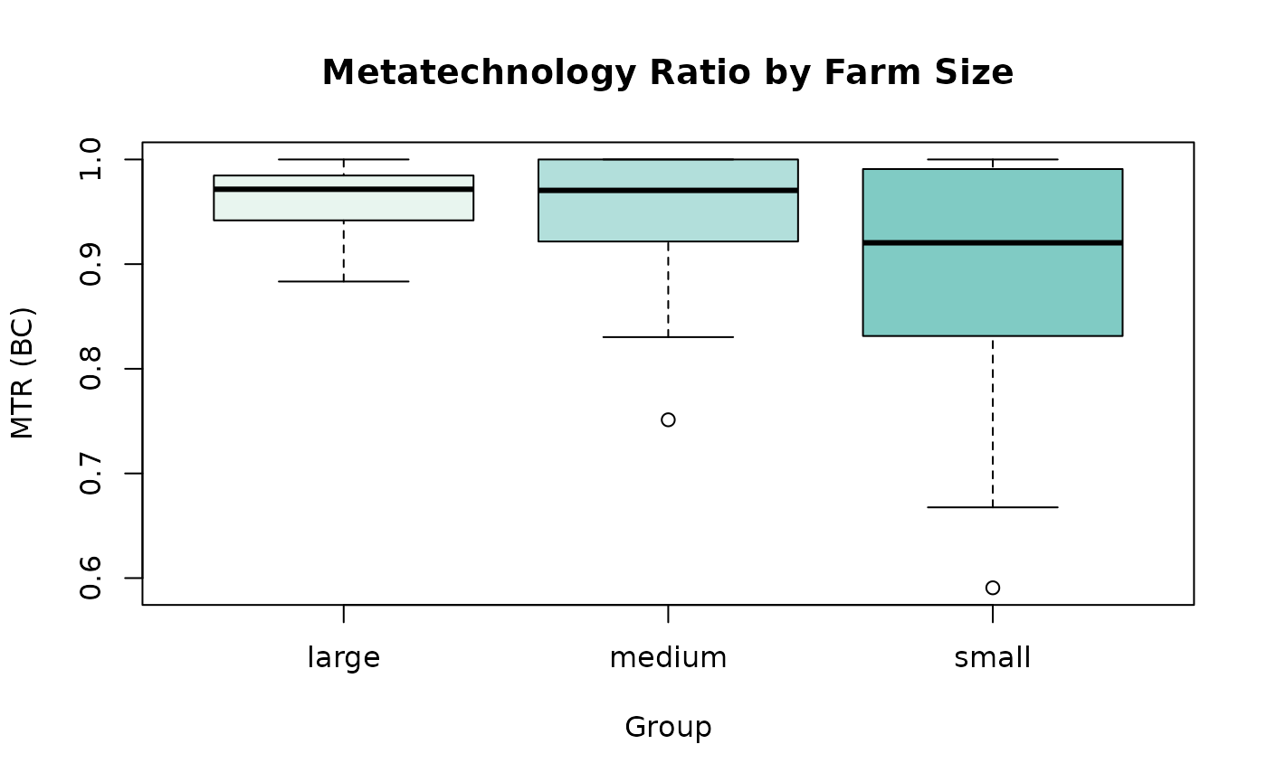
# Histogram of TE_meta_BC
hist(eff$TE_meta_BC, breaks = 30,
     main = "Distribution of Metafrontier TE",
     xlab = "TE_meta_BC", col = "#2d8f65", border = "white")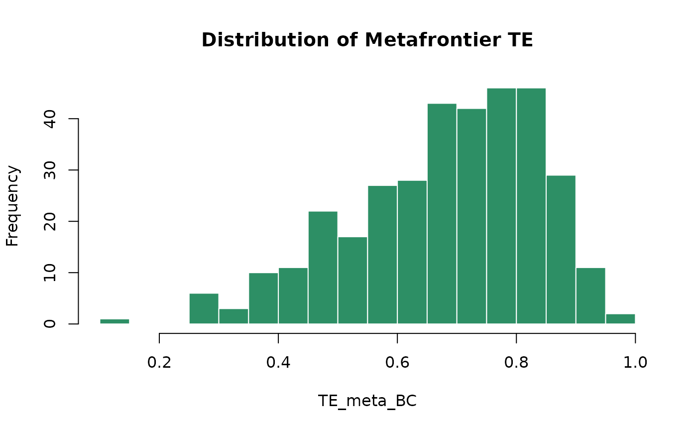
coef() — Estimated Coefficients
Returns the metafrontier coefficient vector (for QP and SFA methods;
NULL for LP).
# First fit a QP model
meta_qp <- smfa(
  formula    = log(PROD) ~ log(AREA) + log(LABOR) + log(NPK),
  data       = ricephil, group = "group", S = 1, udist = "hnormal",
  groupType  = "sfacross", metaMethod = "qp"
)
coef(meta_qp)
Toggle to see the output
#> (Intercept)   log(AREA)  log(LABOR)    log(NPK)
#>  -0.6117795   0.3937843   0.2791273   0.2409454
vcov() — Variance-Covariance Matrix
Returns the variance-covariance matrix of the metafrontier coefficients (for models that estimate metafrontier parameters).
vcov(meta_qp)Toggle to see the output
#>                (Intercept)   `log(AREA)`  `log(LABOR)`    `log(NPK)`
#> (Intercept)   8.514304e-04  1.954064e-04 -1.729963e-04 -3.730091e-05
#> `log(AREA)`   1.954064e-04  5.359537e-05 -3.976453e-05 -9.599635e-06
#> `log(LABOR)` -1.729963e-04 -3.976453e-05  5.962116e-05 -1.454127e-05
#> `log(NPK)`   -3.730091e-05 -9.599635e-06 -1.454127e-05  2.194543e-05
logLik() — Log-Likelihood
Returns the total log-likelihood value of the model (sum of group-level log-likelihoods plus the metafrontier log-likelihood where applicable).
logLik(meta_lp)Toggle to see the output
#> 'log Lik.' -74.28939 (df=18)
ic() — Information Criteria
Returns all three information criteria: AIC, BIC, and HQIC.
ic(meta_lp)#> AIC BIC HQIC
#> 1 184.5788 253.7103 212.113
#> AIC BIC HQIC
#> 1 184.579 253.710 212.113
fitted() — Fitted Values
Returns the fitted frontier values from the model.
Toggle to see the output
#> [1] 2.469286 2.743912 2.626060 1.741342 2.413083 0.838672
residuals() — Residuals
Returns the composite error residuals from the group-level stochastic frontier models.
Toggle to see the output
#> [1] 5.400714 7.606088 7.353940 3.088658 6.326917 1.001328Comparing Multiple Models
You can compare information criteria across methods to select the best model:
meta_lp    <- smfa(log(PROD) ~ log(AREA) + log(LABOR) + log(NPK),
                               data = ricephil, group = "group", S = 1,
                               udist = "hnormal", groupType = "sfacross",
                               metaMethod = "lp")
meta_qp    <- smfa(log(PROD) ~ log(AREA) + log(LABOR) + log(NPK),
                               data = ricephil, group = "group", S = 1,
                               udist = "hnormal", groupType = "sfacross",
                               metaMethod = "qp")
meta_huang <- smfa(log(PROD) ~ log(AREA) + log(LABOR) + log(NPK),
                               data = ricephil, group = "group", S = 1,
                               udist = "hnormal", groupType = "sfacross",
                               metaMethod = "sfa", sfaApproach = "huang")
#> Warning: The residuals of the OLS are right-skewed. This may indicate the absence of inefficiency or
#>   model misspecification or sample 'bad luck'

# Combined information criteria table
models <- list(LP = meta_lp, QP = meta_qp, Huang = meta_huang)
do.call(rbind, lapply(names(models), function(nm) {
  ic_vals <- ic(models[[nm]])
  data.frame(Model = nm, AIC = ic_vals[["AIC"]],
             BIC = ic_vals[["BIC"]], HQIC = ic_vals[["HQIC"]])
}))
Toggle to see the output
#>   Model       AIC       BIC      HQIC
#> 1    LP  184.5788  253.7103  212.1130
#> 2    QP  192.5788  277.0729  226.2318
#> 3 Huang -910.1260 -817.9506 -873.4137