Data Envelopment Analysis with Practical Replication of Results Presented in Sarkis and Talluri (2004)
Introduction
Data Envelopment Analysis (DEA) is a versatile mathematical technique (specifically, linear programming) used for relative performance evaluation and benchmarking in various fields. In this blog, we will explore advanced applications of DEA using the renowned dataset from Sarkis and Talluri (2004). I'll guide you through the process of obtaining the dataset from my GitHub repository, implementing DEA in R using my codes, and comparing the results with those presented in the paper. Let's dive into the world of advanced DEA!
Step 1: Accessing the Dataset
To get started, you can access the dataset from my Github repository, and download the data, file named "e-data.xlsx."
The original source of this environmental data for 48 electric utility plants in the U.S. was from the Energy Information Administration of the United States Department of Energy (EIA). It is a famous dataset that has been utilized severally, including by authors such as Sarkis and Talluri (2004), Tyteca (1998), and Fare et al. (1996).
Step 2: Importing the Data
In R, you can use the readxl library to import Excel data. Here's how to import the dataset:
# Install and load the necessary library
install.packages("readxl")
library(readxl)

# Import the data from the Excel file and call it data
data <- read_excel("e-data.xlsx")
You can use View(data) to inspect the imported dataset and names(data) to see the column names.
Step 3: Importing DEA Results
Next, import the DEA results from the same Excel file, specifically the sheet named "DEA efficiencies":
    # Import DEA results from the Excel file
      dea.data <- read_excel("e-data.xlsx", sheet = "DEA efficiencies")
Again, you can use View(dea.data) to inspect the imported DEA results and names(dea.data) to see the column names.
Step 4: Replicating BCC Results
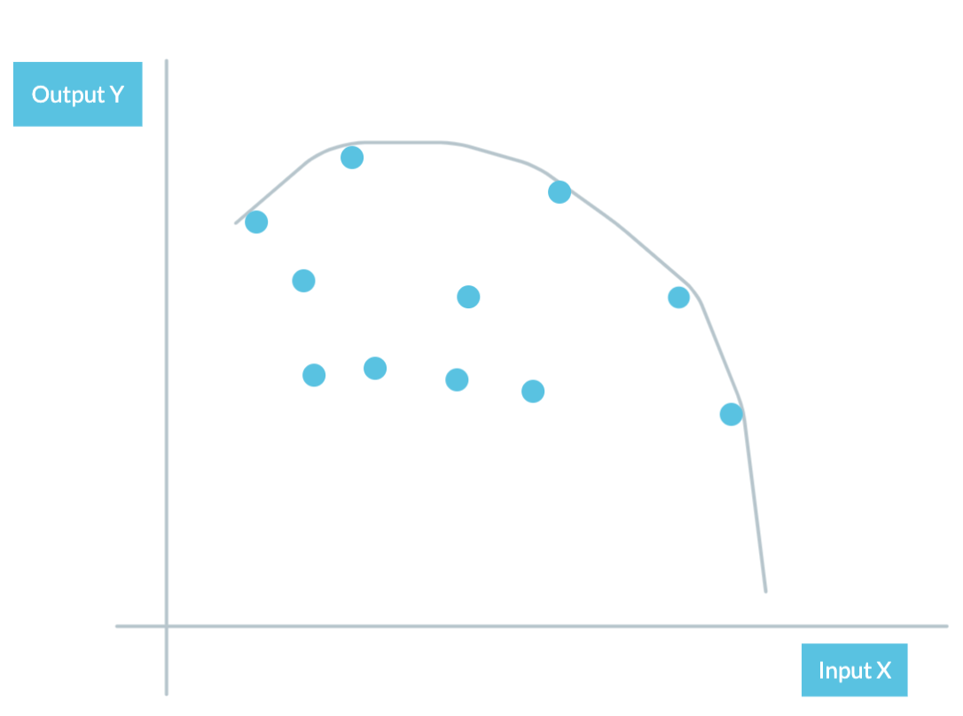
The Banker, Charnes, and Cooper (1984)model allows for estimating efficiency scores under Variable Returns to Scale (VRS). Essentially, VRS is a production concept where a firm's or organization's output doesn't increase proportionally to changes in its inputs. In this case, the production output $y =f(x)$ may increase at a decreasing rate, remain constant, or even decrease when inputs are increased.
Broadly put, changes in the scale of production impact productivity and efficiency. This means that firms operating under VRS may not be at an optimal scale, and they can improve efficiency by adjusting their input levels.
Now, let's replicate the BCC model results from Sarkis and Talluri (2004). We'll use the deaR library for this purpose.
      # Load the deaR library
      library(deaR)

      # Prepare the data for BCC model
      data2 <- data.frame(
      ID = data$`Plant Number`,
      SO2 = data$`SO2 (Tons/yr)`,
      NOx = data$`Nox (Tons/yr)`,
      CO2 = data$`CO2 (Tons/yr)`,
      ENERGY = data$`Energy Input*`,
      LABOUR = data$Labor,
      OUTPUT = data$`Output (MkWh)`)

      # Create a DEA dataset
      dea <- make_deadata(datadea = data2, dmus = 1, ni = 5, no = 1)
      # Create the BCC model
      dea.bcc <- model_basic(dea, dmu_eval = 1:48, dmu_ref = 1:48, orientation = "io", rts = "vrs")
      # Summarize the BCC model
      summary(dea.bcc)

      # Calculate BCC efficiencies
      eff.bcc <- efficiencies(dea.bcc)
      eff.bcc
This code replicates the BCC model as per Sarkis and Talluri (2004) and calculates efficiency scores.
Step 5: Replicating CCR Results
As opposed to the BCC model, the Charnes, Cooper, and Rhodes (1978)(CCR) model assumes constant returns to scale. In essence, this means that when a firm's or organization's inputs increase, its output also increases proportionately. In other words, if you double the inputs (e.g., labor, capital), the output will also double, and vice versa.
The implication of this is that increasing the scale of production doesn't lead to changes in productivity or efficiency. Firms operating under constant returns to scale are typically considered to be at an optimal scale, meaning they are producing at maximum efficiency with their current resource levels.
Similarly, you can replicate the CCR model results:
      # Create a DEA dataset (if not already created)
      dea <- make_deadata(datadea = data2, dmus = 1, ni = 5, no = 1)

      # Create the CCR model
      dea.ccr <- model_basic(dea, dmu_eval = 1:48, dmu_ref = 1:48, orientation = "io", rts = "crs")

      # Summarize the CCR model
      summary(dea.ccr)

      # Calculate CCR efficiencies
      eff.ccr <- efficiencies(dea.ccr)
      eff.ccr
This code replicates the CCR model and calculates efficiency scores.
Step 6: Comparing Results
Finally, you can compare the results you obtained with the DEA results from Sarkis and Talluri (2004) using the following code:
      # Compare BCC and CCR results with the DEA dataset
      cbind(dea.data$BCC, eff.bcc)
      cbind(dea.data$CCR, eff.ccr)
This code compares your DEA results (eff.bcc and eff.ccr) with the values provided in the "DEA efficiencies" sheet of the dataset. You can access
Conclusion
In this blog, I've explored advanced applications of DEA using the Sarkis and Talluri (2004) dataset. I've shown you how to import the data, replicate BCC and CCR models using R and the deaR library, and compare the results with those presented in the paper. DEA is a powerful tool for efficiency analysis, and by following these steps, you can gain hands-on experience in applying DEA to real-world datasets. Happy analyzing!